Matrix Traversal
A grid is one of the most deceptively familiar structures in programming. It looks like a simple 2D array, rows and columns you can loop over, and for plenty of tasks that is all it is. But the moment the question involves connection, "how big is this region," "can I get from here to there," "how many separate blobs are there," the grid reveals its true nature: it is a graph in disguise. Each cell is a node, and its edges are the neighbors it touches, usually the four cells up, down, left, and right, sometimes the diagonals too. Once you see that, every graph traversal you know comes flooding in, and grid problems that felt like a special genre turn out to be BFS and DFS wearing a coordinate system.
The two habits that make grid traversal reliable are both about not tripping over the edges of your own board. First, bounds checking: before you step to a neighbor, confirm the row and column are actually inside the grid, or an index error is waiting. Second, marking visited, because a grid is riddled with cycles (every cell can walk back to the one it came from), so without a memory of where you have been, a flood fill loops forever. A common and tidy trick is to mark visited in place, overwriting a cell as you consume it, which saves an entire parallel visited array.
Flood fill: spread through everything connected
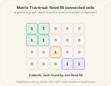
Counting the islands in a grid of land (1) and water (0) is the canonical grid problem. Sweep every cell, and each time you find unclaimed land, launch a DFS that floods the entire connected landmass, marking it so you never count it twice. Each launch is exactly one island.
def num_islands(grid):
    if not grid: return 0
    rows, cols = len(grid), len(grid[0])

    def flood(r, c):
        if r < 0 or r >= rows or c < 0 or c >= cols or grid[r][c] != '1':
            return                                  # off the board, or water, or already sunk
        grid[r][c] = '0'                            # mark visited by consuming it
        flood(r + 1, c); flood(r - 1, c)           # spread to the four neighbors
        flood(r, c + 1); flood(r, c - 1)

    count = 0
    for r in range(rows):
        for c in range(cols):
            if grid[r][c] == '1':                   # a new, untouched island
                flood(r, c)
                count += 1
    return count

grid = [list("11000"), list("11000"), list("00100"), list("00011")]
print(num_islands(grid))                            # 3
The whole thing is O(rows * cols): every cell is visited a constant number of times, because once flooded it becomes water and is never entered again. That single guard, "already visited means stop," is what separates a linear sweep from an infinite loop, and swapping the DFS for a BFS queue changes nothing about the count, only the order cells are consumed.
In the wild: the paint bucket in every image editor
Click the paint-bucket tool in any image editor, click a pixel, and a whole region floods with your chosen color, stopping precisely at the edges where the color changes. That is num_islands with the serial numbers filed off. The canvas is a grid of pixels, "connected" means "adjacent and the same color as where you clicked," and the fill spreads through that connected region exactly the way the flood spreads through an island. The same flood-fill traversal is how computer vision does connected-component labeling: counting cells under a microscope, measuring tumor regions in a medical scan, or grouping the pixels of each detected object in a segmented image.
It is genuinely the same problem, not a lookalike. Islands, paint regions, and image blobs are all "maximal sets of grid cells connected by a same-value rule," and the traversal does not care whether the value is land, a color, or a segmentation label. Recognize the grid-as-graph underneath and a whole visual, spatial category of problems becomes the graph traversal you already know, just with (row, col) coordinates and a neighbor rule instead of an explicit adjacency list.
The trigger
The data is a 2D grid and the question involves regions, paths, or spreading: count the connected areas, find the shortest route through a maze, fill or infect from a starting cell, measure the largest blob. Any "connected cells" or "reach across the grid" phrasing is the tell. If you can describe a cell's neighbors, you have a graph, and grid traversal is the frame.
Where it shows up
- Connected components: counting islands, flood fill and paint bucket, blob labeling in vision, counting enclosed regions.
- Shortest paths on a grid: fewest steps through a maze, shortest path with obstacles, multi-source spread like rotting oranges (BFS).
- Grid dynamic programming: minimum path sum, counting paths, largest square of ones, where the grid is scanned in dependency order.
Where it bites
Off-by-one boundary bugs top the list: check bounds before indexing, not after, or the first neighbor off the edge crashes you. Forgetting to mark visited turns a flood fill into an infinite loop on the very first cycle. And recursion depth is a real limit here, because a single large connected region can nest the DFS thousands of calls deep and overflow the stack; on big grids, an explicit stack or a BFS queue is the safe choice. Deciding whether diagonals count as neighbors is a spec question that quietly changes every answer, so pin it down first.
When it is the wrong tool
If the question is a plain per-cell computation with no notion of connectivity (sum every cell, transform each value), a simple nested loop is the whole job and traversal machinery is overkill. If cells carry different movement costs, unweighted BFS no longer gives the cheapest path and you want Dijkstra or A*. And if you are re-flooding overlapping regions again and again, a single connected-components pass that labels every cell once, or a union-find structure, beats repeated independent traversals.
Its neighbors
Matrix traversal is Graph Traversals with an implicit, coordinate-based adjacency, so BFS gives shortest grid paths and DFS gives flood fill, exactly as on any graph. It shades into Dynamic Programming when the grid is filled in dependency order for path or counting problems, and it shares its explore-and-mark spine with Backtracking whenever the grid search involves trying and undoing moves, as in word search.
References
- Introduction to Algorithms (CLRS), 4th ed., Cormen, Leiserson, Rivest, Stein, 2022
- The Algorithm Design Manual, 3rd ed., Steven Skiena, 2020